| |
|
||||||||||
Wichtiger Hinweis:
Diese Website wird in älteren Versionen von Netscape ohne graphische Elemente dargestellt. Die Funktionalität der Website ist aber trotzdem gewährleistet. Wenn Sie diese Website regelmässig benutzen, empfehlen wir Ihnen, auf Ihrem Computer einen aktuellen Browser zu installieren. Weitere Informationen finden Sie auf
folgender Seite.
Important Note:
The content in this site is accessible to any browser or Internet device, however, some graphics will display correctly only in the newer versions of Netscape. To get the most out of our site we suggest you upgrade to the latest Netscape.
More information
Clustering is probably the most widely used tool in the analysis of gene expression data. Its goal is to find groups of genes that have similar expression patterns. The basic assumption behind clustering approaches is that two genes with similar expression patterns are mechanistically related. Since there are many ways in which these two genes could be related (activation by the same transcription factor, one acting as transcription factor for the other, being involved in the same biological process and therefore regulated similarly by the cell, etc.) analysis of gene expression alone is generally not sufficient to reveal what kind of relation connects the genes. A cluster analysis consists of three main steps: (i) choosing a mathematical representation reflecting the biological question, (ii) identifying an algorithm that solves the mathematical problem which in general means optimizing a score which describes the quality of a cluster or a clustering and (iii) analyzing the results using additional knowledge and data. Choosing a similarity measure is just one part of the first step. A complete mathematical problem formulation also contains a definition of the relation between clusters, e.g., whether clusters should be allowed to overlap.
Looking at the development of clustering algorithms in the last few years one can clearly see a trend to include more and more biological considerations in the problem formulation. Traditional clustering approaches such as k-means and hierarchical clustering put each gene in exactly one cluster. Methods in this category are most widely used and have proven to be useful in many studies. In general, the assumption that all genes behave similarly in all conditions, may be too restrictive. To account for this, biclustering approaches carry out the grouping in both dimensions simultaneously: genes and conditions. This allows to find subgroups of genes that show the same response under a subset of conditions, e.g., if a cellular process is only active under these conditions. Furthermore, if a gene participates in multiple pathways that are differentially regulated, one would expect this gene to be included in more than one cluster; this cannot be achieved by traditional clustering. Several biclustering algorithms have been proposed in the literature, each of which has strengths and weaknesses for the application in different biological scenarios. Accordingly, it can be useful in practice to try different approaches and to choose that algorithm that delivers the best results.
BicAT implements the following biclustering methods: (i) Cheng and Church’s algorithm (CC) which is based on a mean squared residue score (Cheng and Church, 2000); (ii) the Iterative Signature Algorithm (ISA) which searches for submatrices representing fix points (Ihmels et al., 2004); (iii) the Order-Preserving Submatrix Algorithm (OPSM) which tries to identify large submatrices for which the induced linear order of the columns is identical for all rows (Ben-Dor et al., 2003); (iv) the xMotifs algorithm, an iterative search method which seeks biclusters with quasi-constant expression values (Murali and Kasif, 2003); (v) Bimax, an exact biclustering algorithm based on a divide-and-conquer strategy that is capable of finding all maximal bicliques in a corresponding graph-based matrix representation (Prelic et al., 2005). In addition, two standard clustering procedures, namely hierarchical clustering (HCL) and K-means clustering, are included. All references to the cited papers can be found on the publications page.
An analysis of gene expression data starts with the formulation of a biological question. If this question can be answered with finding patterns of gene expression, a clustering approach is sensible. The first step for this analysis would be to prepare the data and visualize them in a human friendly way, e.g. as a heatmap. For the actual analysis, the choice of algorithm and of their specific parameters, like dissimilarity measure, optimization criterion, number of clusters, and search strategy is not easy to make and out of scope of this introduction. For the less experienced user, the default settings of the provided algorithms in BicAT can be used and the choice of algorithm can be made by trying and analyzing the quality of the results. After running one or several algorithms on the data, the clustering results can be searched and filtered for genes of interest. Furthermore, a gene pair analysis, provided by BicAT, can be conducted and the results can be exported for further interpretation with the help of other tools.
This part of the manual describes all functions provided by the BicAT software. If you prefer a step-by-step guide as an introduction, please refer to the tutorial section.
At startup, the main windows appears:
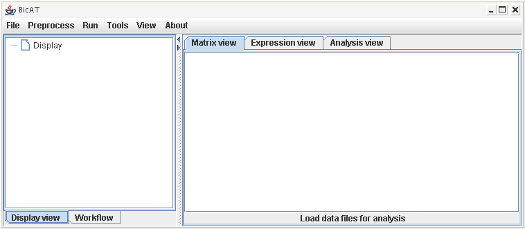
Workspace:
On the left hand side panel, you can identify two tabs: Display View and Workflow. The workflow tab provides a short quickstart guide with the usual analysis steps.
The Display View is the area reserved for the display of loaded data sets and all different results that come out of the analyses. The loaded data sets are organized in a tree-like manner and get a unique number (starting with data set 0). The same data set can be loaded multiple times to conduct different calculation series on the same data while keeping the results organized in different branches of the tree. Every loaded data file gets a branch of it's own in the tree structure in the Display view with all according results of clustering runs, filter and search procedures or from other analysis steps. By clicking on an item inside a specific branch this data set gets selected and is used in all the following calculations until another data set (or result of another data set) gets selected. When the calculation is finished, the data tree collapses to the top level. Branches of the tree can be deleted by right-clicking them and choosing "delete node".
On the right hand side panel, three tabs are provided:
Main menu:
File: Open files and export results
Preprocess: Normalize, discretize and logarithmize data
Run: Cluster and bicluster
Tools: Postprocess the data, i.e. search, filter for genes or conditions and perform gene pair analysis
View: Zooming the view and limiting the display to keep large matrices manageable
About: Information about copyright and authorship
In the following, the important menu items are described in detail:
To load input data, choose:
File -> Load ... -> Expression Data
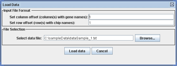
A dialog appears where you can specify the row and column offset. This is important to extract the names of the genes and of the conditions. The default value for the offsets is 1, indicating that the matrix has a single header column (gene identifiers), and a single header row (names of conditions). If there are more than one according rows or columns, please specify this here. The data set has to be provided as a plain text file. All fields in the file have to be separated by tabs. Blanks in the names will be omitted during import of the file.
If you are planning to analyze a large data set (larger then 5 megabytes of data), please refer to the special tips for starting BicAT on Windows system.
Preprocess -> Preprocess data
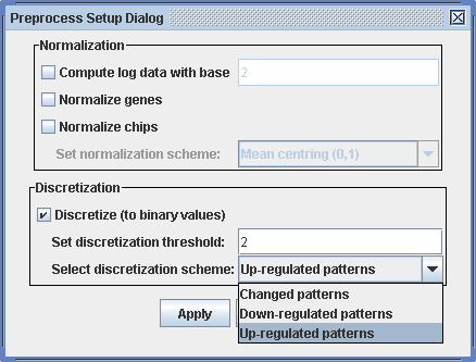
A dialog appears where you can choose to:
Discretization of the input matrix is important only if you intend to use the BiMax algorithm, which works exclusively with discrete (binary) matrices. The preprocessed and the discretized data sets are visualized in the according items of the data display in the tree in the Display view. The spots in the heat map change accordingly. After preprocessing all the following calculations are done with the preprocessed data.
Every clustering algorithm need different parameters to run. The given default parameters should provide reasonable results. A detailed description of each parameter can be found in the according publication.
Run -> Biclustering BiMax
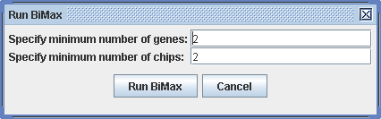
The dialog asks you to specify the minimum for the gene and chip numbers of the biclusters. By specifying larger lower bounds, fewer biclusters will be returned, which reduces the time for the calculation.
Run -> Biclustering CC
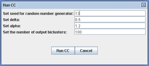
For CC, xMotifs and ISA algorithms, a dialog appears for the parameters that are needed for the algorithm. Detailed information about each parameter can be found in the corresponding literature on the publications section. The default parameters should yield reasonably results. Only the number of output biclusters can be set to a higher number if enough computation resources is available.
The clustering algorithms provided within BicAT are Hierarchical clustering and K-means clustering. The implementations allow to choose between different parameter settings. The implementations of the clustering algorithms are standard implementations comparable, e.g., to what is provided in mathematical programming packages like MATLAB.
Run -> Clustering HCL
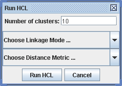
For Hierachical clustering, there are different settings for the linkage mode and for the distance metric available. For the linkage mode, single, average and complete linkage is possible. For the distance metric, a collection of established metrics is provided. For an introduction into this field, see the literature on the publications page.
Run -> Clustering K-means
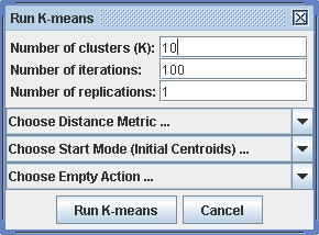
For K-means the number of clusters, iterations and replications can be reduced to keep calculation time feasible. In addition to the distance metric, the start mode and the action on finding empty clusters has to be specified.
The post-processing tools asks you to specify which list of clusters you would like to analyze. This can be an initial result of a (bi-)clustering run or a result of a previous post-processing step. After selecting a list in the pulldown menu the parameters for the choosen tool have to be specified.
Naming convention for the data sets:
D0: Data set number 0
The number increases when you load more than one data set.
Naming convention for the (bi-)cluster lists:
L.0: List of biclusters (i.e. result from a biclustering run)
C.0: Cluster list (i.e. result from a clustering run)
S.0: Search results
F.0: Filter results
A.0: Analysis results from the gene pair analysis
The number increases if you make more than one operation of the same type.
Tools -> Search Results
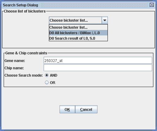
Criteria for the search are a specific gene and/or a specific condition of special interest. Searches can be executed in two modi: and finds biclusters containing the specified gene and the specified chip, while or finds biclusters, where at least either of the gene or chip need to be present.
Tools -> Filter Results
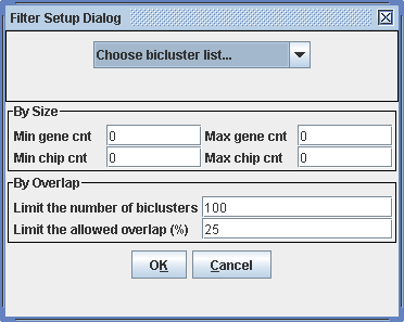
The filtering procedure allows you to select only those biclusters satisfying certain size constraints. You can specify lower and upper bounds on gene and condition numbers in the bicluster. Furthermore, it is possible to select only a number of the largest biclusters from a specific run, and simultaneously ensure that the selected biclusters do not overlap at a large extent (i.e. by Overlap).
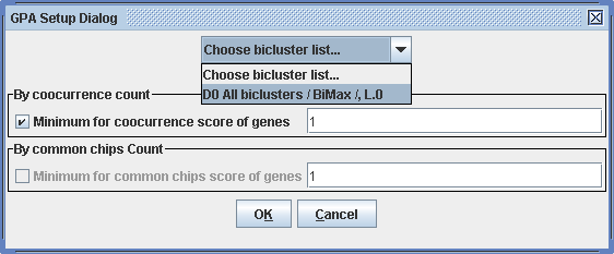
This procedure allows to score gene pairs, according to the frequency with that these appear together in one bicluster. The minimum for cooccurrence in a bicluster and for the number of common chips count can be specified. The scores can then be viewed in the right hand panel by clicking on the corresponding analysis result in the tree in the Display view and afterwards selecting the Analysis view tab on the right panel of the workspace. The list of the gene pairs with the respective scores can be exported for visualization by external tools, for example, BioLayout of EBI UK.
File -> Export -> ...
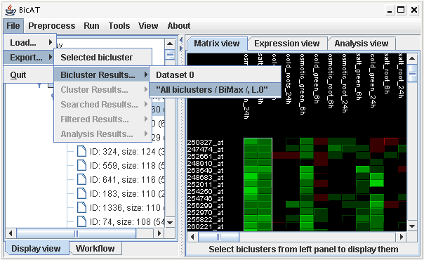
All results can be exported to plain text files. To export a single bicluster, select it and choose Export->selected bicluster. For whole lists of (bi-)clusters or for results from filter, search or gene pair analyses, select the corresponding submenu and then the result list under the name of the data set. The lists of biclusters are named referring to the naming conventions.
Back to the BicAT main page.

")