BicAT Tutorial

This tutorial provides a step-by-step walkthrough for a biclustering analysis with the BicAT Toolbox.

1. Load a data set

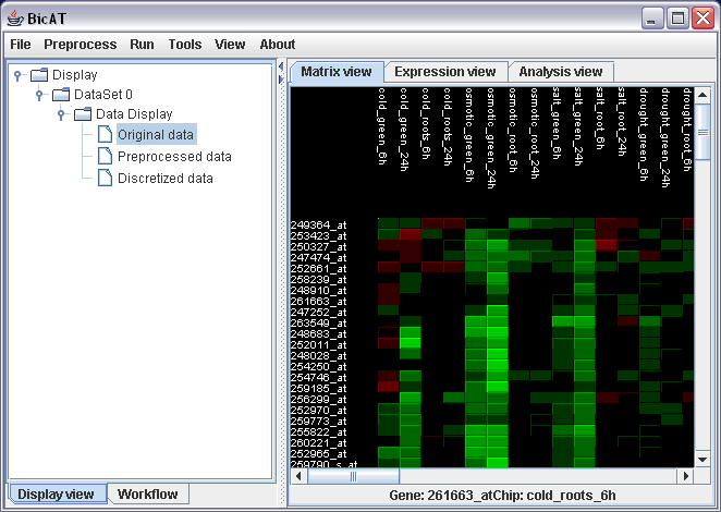
After downloading BicAT, open it by double clicking the BicAT_v2.2.jar file (windows) or run the program by typing ./run_solaris or ./run_linux. If this does not work, please refer to the installation guide. Load the data set by selecting File -> load... -> Expression Data in the menu. Select Browse... and choose dataSample_1.txt in the sampleData folder of the BicAT distribution. Leave the row and column offset to 1 for there is one line and one row with chip respectively gene names in the provided sample data set. You should now see this picture:

2. Preprocess the data

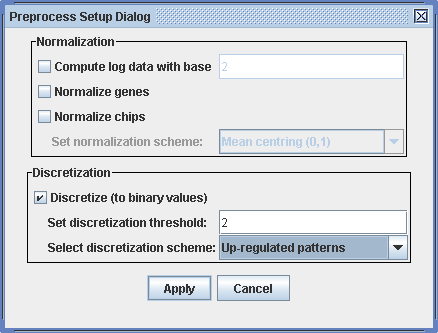
We want to run the bimax biclustering algorithm on the data. Therefore, we need to discretize the data to binary values. Select Preprocess -> Preprocess data in the menu. The data in the dataSample_1.txt file is already normalized. So all we have to do here is to discretize them. To do this, click the button for discretization in the lower part of the preprosess dialog. In this analysis, we are interested only in genes that are up-regulated due to our experiments. So choose up-regulated patterns in the pull-down menu for the discretization scheme. Leave the discretization threshold as it is as "2" is a reasonable threshold for this data set. All expression values above this threshold will be turned to one (red in the matrix view), all others to zero (green).

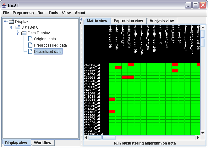
In the matrix view, you can now see the discretized matrix. Click on "Discretized data" in the Data Display branch in the left panel.

3. Run biclustering analysis

To run the bimax algorithm on the data, choose Run -> Biclustering BiMax in the menu. One advantage of the bimax algorithm is that it finds all existing biclusters. But you can also limit the number of found biclusters, by setting the minima for rows and columns to a higher value. Leave the minima as it is and click "Run BiMax". Two messages appear giving you feedback of starting and finishing of the calculation process. (If the calculation is very fast, these can appear in the wrong order). To look at the results, expand the branch of "dataSet 0" to Bicluster results and select a bicluster out of the bicluster list under "All biclusters"

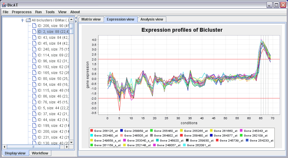
The Expression view displays the expression profile of the selected bicluster. Click on the Expression view tab in the right panel. The colored curves stand for expression values of single genes in the cluster over all conditions in the data set. The upright grey bars on the right mark the conditions that are included in the bicluster. The red lines mark the discretization threshold.

4. Filter and search the biclustering results

If our list of biclusters is too large, we can reducing it to more interesting, i.e. larger, biclusters by selecting Tools -> FIlter biclusters. You can either specify a minimum for the number of genes and chips or take limit the list to a specific number of the largest clusters.

Normally, one is interested in a specific gene. We can use the search function of BicAT to see with what other genes our gene of interest is up-regulated in the same experiments . Say we are interested in a gene with the name "248606_at". We search our list of biclusters by choosing Tools -> search biclusters in the menu and typing in the name of the gene of interest in the Search Setup Dialog. Don't forget to choose the list of biclusters.

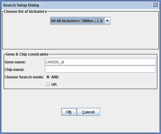
After clicking "OK" the search results can be found by expanding the branch of our data set and selecting the "Search result" branch.

5. Perform a gene pair analysis

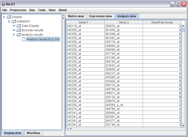
The gene pair analysis provides a way to look with what other genes a gene of interest is involved in a bicluster. To run a gene pair analysis, select Gene Pair Analysis in the tools menu. In the following dialog choose our bicluster list from the bimax run in the pull-down menu, leave the modus to "By cooccurrence count" and leave the minimum for cooccurence to 2. By expanding the data set in the display view to Analysis results, clicking on the "Analysis result of L0" and finally selecting the Analysis view on the right hand panel, we get a table with all Gene pair scores of all genes that occur to be in the same bicluster with another gene at least twice. The results can be sorted by clicking on the label, e.g. "Gene 1" to look for specific genes of interest or "GenePair Score" to look for the genes with the most connections to other genes.

6. Export results

We want to export the following results: (i) a complete list of found biclusters of the bimax run, (ii) the biclusters that contain our specific gene of interest "248606_at" and (iii) the analysis results of the gene pair analysis.

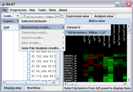
(i) Select File -> Export... -> Biclustering results -> "All biclusters / BiMax /, L.0" and specify where you want to save the text file. The text file yields the ID numbers of the biclusters, and the genes and conditions of the individual biclusters in separate lines.

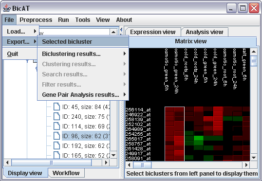
(ii) For saving the gene lists of a specific biclusters containing a gene of interest select the bicluster in the Bicluster results branch and select File -> Export... -> Selected bicluster and specify the place to save the text file with the gene and chip names.

(iii) For exporting the results of a gene pair analysis simply select File -> Export... -> Gene Pair Analysis results -> "Analysis results of L.0, A.0". The resulting text file yields four columns for Gene 1, Gene 2, gene pair score and a fourth column with the Graph Distance. This column yields only ones but is required for compatibiliy reasons with programs like BioLayout of EBI UK.

Back to the BicAT main page.